Schöne Matrizen mit nicematrix
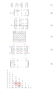
Um ansprechende Matrizen zu setzen gibt es mit dem nicematrix Paket ein recht neues Paket, das sich alle anschauen sollten, die viel mit Matrizen zu tun haben. Die folgenden Beispiele sind der Dokumentation entnommen, teilweise braucht man mehrere LaTeX-Läufe für das finale Ergebnis.
%!TEX TS-program = Arara % arara: pdflatex: {shell: yes} \documentclass[12pt,ngerman]{scrartcl} \usepackage[utf8]{inputenc} \usepackage[T1]{fontenc} \usepackage{babel} \usepackage{xcolor} \usepackage{tikz} \usepackage{siunitx} \usepackage{nicematrix} \NiceMatrixOptions{cell-space-top-limit = 1pt,cell-space-bottom-limit = 1pt} \begin{document} \begin{equation} \begin{pmatrix} \frac12 & -\frac12 \\ \frac13 & \frac14 \\ \end{pmatrix} = \begin{pNiceMatrix} \frac12 & -\frac12 \\ \frac13 & \frac14 \\ \end{pNiceMatrix} \end{equation} \begin{equation} A = \begin{pNiceMatrix}[baseline=2] \frac{1}{\sqrt{1+p^2}} & p & 1-p \\ 1 & 1 & 1 \\ 1 & p & 1+p \end{pNiceMatrix} \end{equation} \NiceMatrixOptions{cell-space-top-limit=1pt,cell-space-bottom-limit=1pt} \begin{equation} A=\begin{pNiceArray}{cc|cc}[baseline=line-3] \dfrac1A & \dfrac1B & 0 & 0 \\ \dfrac1C & \dfrac1D & 0 & 0 \\ \hline 0 & 0 & A & B \\ 0 & 0 & D & D \\ \end{pNiceArray} \end{equation} \begin{equation} \begin{NiceArray}{*{5}{c}}[hvlines] \diagbox{x}{y} & e & a & b & c \\ e & e & a & b & c \\ a & a & e & c & b \\ b & b & c & e & a \\ c & c & b & a & e \end{NiceArray} \end{equation} \NiceMatrixOptions{code-for-first-row = \color{red}, code-for-first-col = \color{blue}, code-for-last-row = \color{green}, code-for-last-col = \color{magenta}} \begin{equation} \begin{pNiceArray}{cc|cc}[first-row,last-row=5,first-col,last-col,nullify-dots] & C_1 & \Cdots & & C_4 & \\ L_1 & a_{11} & a_{12} & a_{13} & a_{14} & L_1 \\ \Vdots & a_{21} & a_{22} & a_{23} & a_{24} & \Vdots \\ \hline & a_{31} & a_{32} & a_{33} & a_{34} & \\ L_4 & a_{41} & a_{42} & a_{43} & a_{44} & L_4 \\ & C_1 & \Cdots & & C_4 & \end{pNiceArray} \end{equation} \begin{equation} \begin{pNiceArray}{ScWc{1cm}c}[nullify-dots,first-row] {C_1} & \Cdots & & C_n \\ 2.3 & 0 & \Cdots & 0 \\ 12.4 & \Vdots & & \Vdots \\ 1.45 \\ 7.2 & 0 & \Cdots & 0 \end{pNiceArray} \end{equation} \[\begin{NiceMatrix}[ code-before = { \tikz \draw [fill = red!15] (row-7-|col-4) -- (row-8-|col-4) -- (row-8-|col-5) -- (row-9-|col-5) -- (row-9-|col-6) |- cycle ; } ]1 \\ 1 & 1 \\ 1 & 2 & 1 \\ 1 & 3 & 3 & 1 \\ 1 & 4 & 6 & 4 & 1 \\ 1 & 5 & 10 & 10 & 5 & 1 \\ 1 & 6 & 15 & 20 & 15 & 6 & 1 \\ 1 & 7 & 21 & 35 & 35 & 21 & 7 & 1 \\ 1 & 8 & 28 & 56 & 70 & 56 & 28 & 8 & 1 \end{NiceMatrix}\] \( \begin{bNiceMatrix} C[a_1,a_1] & \Cdots & C[a_1,a_n] & \hspace*{20mm} & C[a_1,a_1^{(p)}] & \Cdots & C[a_1,a_n^{(p)}] \\ \Vdots & \Ddots & \Vdots & \Hdotsfor{1} & \Vdots & \Ddots & \Vdots \\ C[a_n,a_1] & \Cdots & C[a_n,a_n] & & C[a_n,a_1^{(p)}] & \Cdots & C[a_n,a_n^{(p)}] \\ \rule{0pt}{15mm} & \Vdotsfor{1} & & \Ddots & & \Vdotsfor{1} \\ C[a_1^{(p)},a_1] & \Cdots & C[a_1^{(p)},a_n] & & C[a_1^{(p)},a_1^{(p)}] & \Cdots & C[a_1^{(p)},a_n^{(p)}] \\ \Vdots & \Ddots & \Vdots & \Hdotsfor{1} & \Vdots & \Ddots & \Vdots \\ C[a_n^{(p)},a_1] & \Cdots & C[a_n^{(p)},a_n] & & C[a_n^{(p)},a_1^{(p)}] & \Cdots & C[a_n^{(p)},a_n^{(p)}] \end{bNiceMatrix} \) \end{document} |