ASNs (Archive Serial Numbers) in LaTeX erzeugen
Ich experimentiere aktuell mit paperless-ngx, in der c’t war eine passende Anleitung für Docker auf Synology NAS, der ich gefolgt bin.
Um Bögen mit Archive Serial Numbers zu erstellen, will ich natürlich LaTeX nutzen, ticket.sty heißt hier das Zauberwort. (Es gibt auch web-basierte Generatoren, siehe https://tobiasmaier.info/asn-qr-code-label-generator/)
Anbei der Quellcode für LaTeX, für den Druck auf andere Bögen als Avery Zweckform 4736 muss man das Format der Labels anpassen. Dann ist die LaTeX-Datei zweimal zu übersetzen.
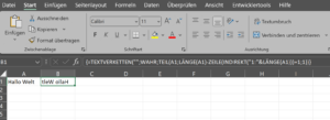
\documentclass[a4paper,12pt]{scrartcl} \usepackage[total={210mm,297mm},top=0mm,left=0mm,bottom=0mm,includefoot]{geometry} \usepackage[ASN]{ticket} %boxed,cutmark during development \usepackage{qrcode} \usepackage{forloop} \usepackage[T1]{fontenc} % https://tex.stackexchange.com/questions/716116/generate-sequential-padded-barcodes-with-qrcode?noredirect=1#comment1780003_716116 \makeatletter \newcommand{\padnum}[2]{% \ifnum#1>1 \ifnum#2<10 0\fi \ifnum#1>2 \ifnum#2<100 0\fi \ifnum#1>3 \ifnum#2<1000 0\fi \ifnum#1>4 \ifnum#2<10000 0\fi \ifnum#1>5 \ifnum#2<100000 0\fi \ifnum#1>6 \ifnum#2<1000000 0\fi \ifnum#1>7 \ifnum#2<10000000 0\fi \ifnum#1>8 \ifnum#2<100000000 0\fi \ifnum#1>9 \ifnum#2<1000000000 0\fi \fi\fi\fi\fi\fi\fi\fi\fi\fi \expandafter\@firstofone\expandafter{\number#2}% } \makeatother \begin{filecontents*}[overwrite]{ASN.tdf} \unitlength=1mm \hoffset=-16mm \voffset=-8mm \ticketNumbers{4}{12} \ticketSize{45.7}{21.2} % Breite und Höhe der Labels in mm \ticketDistance{2.5}{0} % Abstand der Labels \end{filecontents*} %reset background \renewcommand{\ticketdefault}{}% \newcounter{asn} % start value of the labels \setcounter{asn}{1} \newcommand{\mylabel}{ \ticket{% \hspace*{4mm}\raisebox{9mm}[4mm][2mm]{% \qrcode[height=1.4cm]{ASN\padnum{5}{\value{asn}}}% ~\texttt{\large ASN\padnum{5}{\value{asn}}} } \stepcounter{asn} } } \begin{document} % just for the loop \newcounter{x} % create 48 labels \forloop{x}{1}{\value{x} < 49}{ \mylabel% } %print on Avery Zweckform 4736 % in original size, not scaled to fit page \end{document} |