Archive for the ‘Allgemein’ Category.

dbt and the ECB f/x Rates – Part 2

This entry is Teil 2 von 3 in the series dbt - ECB FX Example

In this article we will continue our dbt journey. With dbt-core installed we can ask dbt to set up a new project for us.

Simply go to the root folder where your project folder shall be created and run dbt init projectname. dbt will then ask you for the database adapter and the connection settings as well as for the schema dbt is to build its objects in.

After these questions and answers dbt tells you that you may run dbt debug now to check if everything is fine, BUT: you need to switch first to the subdirectory you created otherwise there will be a meaningless error message:


Encountered an error:
Internal Error
Profile should not be None if loading profile completed

If run in the correct subdirectory dbt debug should not produce any errors. If it does, run the error message through the search engine of your choice.

C:\Users\UWe\Desktop\fx_project>dbt debug
16:52:20  Running with dbt=1.10.13
16:52:20  dbt version: 1.10.13
16:52:20  python version: 3.12.6
16:52:20  python path: C:\Python312\python.exe
16:52:20  os info: Windows-11-10.0.26200-SP0
16:52:20  Using profiles dir at C:\Users\UWe\.dbt
16:52:20  Using profiles.yml file at C:\Users\UWe\.dbt\profiles.yml
16:52:20  Using dbt_project.yml file at C:\Users\UWe\Desktop\fx_project\dbt_project.yml
16:52:20  adapter type: postgres
16:52:20  adapter version: 1.9.1
16:52:20  Configuration:
16:52:20    profiles.yml file [OK found and valid]
16:52:20    dbt_project.yml file [OK found and valid]
16:52:20  Required dependencies:
16:52:20   - git [OK found]

16:52:20  Connection:
16:52:20    host: localhost
16:52:20    port: 5432
16:52:20    user: postgres
16:52:20    database: FX
16:52:20    schema: dbt
16:52:20    connect_timeout: 10
16:52:20    role: None
16:52:20    search_path: None
16:52:20    keepalives_idle: 0
16:52:20    sslmode: None
16:52:20    sslcert: None
16:52:20    sslkey: None
16:52:20    sslrootcert: None
16:52:20    application_name: dbt
16:52:20    retries: 1
16:52:20  Registered adapter: postgres=1.9.1
16:52:20    Connection test: [OK connection ok]

16:52:20  All checks passed!

In the project folder you find a set of subfolders, remove the models/example subfolder, as it may cause error messages.

Next we will create some basic models, using YAML files.

In models, create sources.yml with the following content:

version: 2
sources:
  - name: raw
    schema: raw
    tables:
      - name: ecb_fx_rates

In models, create a subfolder staging and add stg_fx_rates.sql to this staging subfolder with the following content:

{{ config(materialized='view') }}
SELECT
    fx_date,
    currency,
    rate,
    created_at
FROM {{ SOURCE('raw', 'ecb_fx_rates') }}

This will simply select all the data we have in our raw DB schema.

Next comes is the interesting part. Each row gets a valid_from and valid_to date using a window function.

In models, create a subfolder marts and add fx_rates_with_validity.sql to this marts subfolder with the following content:

{{ config(materialized='table') }}
 
WITH base AS (
    SELECT
        fx_date,
        currency,
        rate
    FROM {{ REF('stg_fx_rates') }}
),
 
with_validity AS (
    SELECT
        currency,
        fx_date                        AS valid_from,
        -- valid_to is the day before the next rate, or null if it's the latest
        lead(fx_date) OVER (
            partition BY currency
            ORDER BY fx_date
        ) - INTERVAL '1 day'             AS valid_to,
        rate,
        -- flag the currently active rate
        CASE
            WHEN lead(fx_date) OVER (
                partition BY currency ORDER BY fx_date
            ) IS NULL THEN TRUE
            ELSE FALSE
        END                              AS is_current
    FROM base
)
 
SELECT * FROM with_validity
ORDER BY currency, valid_from

This will give uzs data as the following

currency valid_from valid_to rate_vs_eur is_current
USD 2025-01-02 2025-01-02 1.0312 false
USD 2025-01-03 2025-01-05 1.0345 false
USD 2025-01-04 null 1.0821 true

It also makes sense now to add some data checks.

In models, create schema.yml with the following content:

version: 2

models:
  - name: stg_fx_rates
    columns:
      - name: rate_date
        tests: [not_null]
      - name: currency
        tests: [not_null]
      - name: rate_vs_eur
        tests: [not_null]

  - name: fx_rates_with_validity
    columns:
      - name: currency
        tests: [not_null]
      - name: valid_from
        tests: [not_null]
      - name: is_current
        tests: [not_null]

We can now run the whole setup:

dbt run
dbt test
dbt docs generate
dbt docs serve

Going forward

Since ECB publishes the latest rate every data at around 16:00 CET the Python job to fetch them should be run each day (apparently after 16:00 CET). Once the raw database is updated you can update the dbt models:

dbt run --select stg_fx_rates fx_rates_with_validity
dbt test --select stg_fx_rates fx_rates_with_validity

In the final part of the series we will add another data market for the latest rates.

dbt and the ECB f/x Rates – Part 1

This entry is Teil 1 von 3 in the series dbt - ECB FX Example

I have recently found the necessity to deal with dbt and Snowflake. As I learn best by practically doing something I decided to write a few practical use cases. Privately I will focus on Postgres SQL as I am not sure about Snowflake’s free tier. What is this dbt? dbt (data build tool) is a commandline tool based on Python that take care of the „T“ in „ETL“, the transformation of data in a data warehouse using SQL. dbt does not care about how you get the raw data into the (raw) DWH, this is not in its scope. dbt-core is available for free (Therefore I will focus on dbt-core, for production environments the paid tiers are most likely more suitable).

In this first example we will download the ECB fx rates from the European Central Bank and play a bit with them by transforming them and creating some data marts.

As mentioned I will use Postgres locally on my machine, so the installation of Postgres on my Windows machine was step 1. To deal with Postgres I can recommend HeidiSQL, does the trick.

Step 2 was the installation of dbt in Python. (Note that I had issues with Python 3.14, I downgraded to Python 3.12)

Besides dbt-core we need the postgres-Adapter dbt-postgres, so pip install dbt-core dbt-postgres helped. I usually do not need virtual environments, so I just installed it globally. We also need the Postgres library and lxml and requests for the ingestion of the XML file:

pip install requests psycopg2-binary lxml

As mentioned dbt does not care how you load the raw data, so with the help of some AI-tool I got the following Python Code to load the 90-days F/X rates file from the European Central Bank.

import requests
import xml.etree.ElementTree as ET
from datetime import datetime
import psycopg2
from psycopg2.extras import execute_values
 
ECB_URL = "https://www.ecb.europa.eu/stats/eurofxref/eurofxref-hist-90d.xml"
 
DB_CONFIG = {
    "host": "localhost",
    "port": 5432,
    "dbname": "FX",
    "user": "postgres",
    "password": "<meingeheimespasswort>",
}
 
def fetch_ecb_fx():
    r = requests.get(ECB_URL, timeout=30)
    r.raise_for_status()
    root = ET.fromstring(r.content)
    ns = {
        "gesmes": "http://www.gesmes.org/xml/2002-08-01",
        "def": "http://www.ecb.int/vocabulary/2002-08-01/eurofxref",
    }
 
    rows = []
 
    # Find Cube with time attribute
    for cube in root.findall(".//def:Cube[@time]", ns):
        fx_date = cube.attrib["time"]
 
        for rate in cube.findall("def:Cube", ns):
            rows.append(
                (
                    fx_date,
                    rate.attrib["currency"],
                    float(rate.attrib["rate"]),
                )
            )
 
    return rows
 
 
def init_db(conn):
    with conn.cursor() as cur:
        cur.execute(
            """
            CREATE SCHEMA IF NOT EXISTS raw;
 
            CREATE TABLE IF NOT EXISTS raw.ecb_fx_rates (
                fx_date date NOT NULL,
                currency varchar(3) NOT NULL,
                rate numeric(20,10) NOT NULL,
                created_at timestamp default now(),
                PRIMARY KEY (fx_date, currency)
            );
            """
        )
    conn.commit()
 
 
def upsert_rates(conn, rows):
    sql = """
        INSERT INTO raw.ecb_fx_rates (fx_date, currency, rate)
        VALUES %s
        ON CONFLICT (fx_date, currency)
        DO UPDATE SET rate = EXCLUDED.rate;
    """
 
    with conn.cursor() as cur:
        execute_values(cur, sql, rows)
 
    conn.commit()
 
 
def main():
    rows = fetch_ecb_fx()
    print(f"Fetched {len(rows)} FX rates")
 
    conn = psycopg2.connect(**DB_CONFIG)
 
    try:
        init_db(conn)
        upsert_rates(conn, rows)
        print("Load complete")
    finally:
        conn.close()
 
 
if __name__ == "__main__":
    main()

When this code is run it should provide some output close to the following.


Fetched 1798 FX rates
Load complete

In the second part of this series we will take care of the dbt work.

Aktenordner in TikZ

Hier ein Beispiel, wie man mit TikZ einen Aktenordner in TikZ zeichnen kann.

\documentclass[tikz,border=5pt]{standalone}
\begin{document}
\begin{tikzpicture}[line join=round, line cap=round]
 
% ------------------------------
% Parameter
% ------------------------------
\def\ordnerwidth{2.5}   % Rückenbreite des Ordners
\def\ordnerheight{11}   % Höhe des Ordners
 
% Abgeleitete Maße
\pgfmathsetmacro{\lochdiam}{0.7*\ordnerwidth}
\pgfmathsetmacro{\labelwidth}{0.8*\ordnerwidth}
\pgfmathsetmacro{\lochx}{0.5*\ordnerwidth}
\pgfmathsetmacro{\labelx}{0.5*(\ordnerwidth-\labelwidth)}
 
% ------------------------------
% Zeichnung
% ------------------------------
 
% Rücken
\draw[fill=gray!20] (0,0) rectangle (\ordnerwidth,\ordnerheight);
 
% Etikettfeld (mittig auf Rücken)
\draw[fill=white] (\labelx,3) rectangle ++(\labelwidth,7);
\foreach \y in {8.5,8,7.5,7,6.5} {
  \draw (\labelx+0.2,\y) -- (\labelx+\labelwidth-0.2,\y);
}
 
% Griffloch (mittig unten am Rücken)
\draw[fill=black!40] (\lochx,1.2) circle (\lochdiam/2);
\draw[fill=white] (\lochx,1.2) circle (\lochdiam/2.2);
 
\end{tikzpicture}
\end{document}

Und hier der Code für den Ordner in 3D:

\documentclass[tikz,border=5pt]{standalone}
\begin{document}
\begin{tikzpicture}[line join=round, line cap=round]
 
% ------------------------------
% Parameter
% ------------------------------
\def\ordnerwidth{2.5}   % Rückenbreite des Ordners
\def\ordnerheight{10}   % Höhe
\def\depth{2}           % Tiefe in die Perspektive
 
% Abgeleitete Maße
\pgfmathsetmacro{\lochdiam}{0.8*\ordnerwidth}
\pgfmathsetmacro{\labelwidth}{0.8*\ordnerwidth}
\pgfmathsetmacro{\lochx}{0.5*\ordnerwidth}
\pgfmathsetmacro{\labelx}{0.5*(\ordnerwidth-\labelwidth)}
 
% ------------------------------
% Zeichnung
% ------------------------------
 
% Rückseite (Rücken sichtbar)
\draw[fill=gray!20] (0,0) -- (\ordnerwidth,0) -- (\ordnerwidth,\ordnerheight) -- (0,\ordnerheight) -- cycle;
 
% Seitenfläche
\draw[fill=gray!10] (\ordnerwidth,0) -- (\ordnerwidth+\depth,0.6) -- (\ordnerwidth+\depth,\ordnerheight+0.6) -- (\ordnerwidth,\ordnerheight) -- cycle;
 
% Oberseite
\draw[fill=gray!30] (0,\ordnerheight) -- (\ordnerwidth,\ordnerheight) -- (\ordnerwidth+\depth,\ordnerheight+0.6) -- (\depth,\ordnerheight+0.6) -- cycle;
 
% Etikettfeld (mittig auf Rücken)
\draw[fill=white] (\labelx,6) rectangle ++(\labelwidth,3);
\foreach \y in {8.5,8,7.5,7,6.5} {
  \draw (\labelx+0.2,\y) -- (\labelx+\labelwidth-0.2,\y);
}
 
% Griffloch (mittig unten am Rücken)
\shade[ball color=black!50] (\lochx,1.2) circle (\lochdiam/2);
\fill[white] (\lochx,1.2) circle (\lochdiam/2.5);
 
% Umrandung
\draw[thick] (0,0) -- (\ordnerwidth,0) -- (\ordnerwidth+\depth,0.6) -- (\ordnerwidth+\depth,\ordnerheight+0.6) -- (\depth,\ordnerheight+0.6) -- (0,\ordnerheight) -- cycle;
 
\end{tikzpicture}
\end{document}

Outer Apply und Cross Apply in SQL nutzen – Die Datenmenge bauen

This entry is Teil 2 von 3 in the series Outer Apply und Cross Apply

Wir kennen jetzt das Problem, nun können wir uns an die Lösung wagen! In diesem Blogbeitrag werden wir alles vorbereiten, was wir für das anschließende „Forward Filling“ der Daten brauchen.

Im ersten Schritt bestimmen wir für die einzelnen Verträge die Monatsendwerte von Start des jeweiligen Vertrags bis zu dessen Ende. Dazu nutze ich den den folgenden rekursiven CTE (Common Table Expression)

WITH MonthSequence AS (
    SELECT
        c.ContNo,
        EOMONTH(c.StartDate) AS MonthEnd,
        c.EndDate
    FROM Contracts c
    UNION ALL
    SELECT
        ms.ContNo,
        EOMONTH(DATEADD(MONTH, 1, ms.MonthEnd)),
        ms.EndDate
    FROM MonthSequence ms
    WHERE EOMONTH(DATEADD(MONTH, 1, ms.MonthEnd)) <= ms.EndDate
)

Das erzeugt uns die folgende Sequenz:

ContNo MonthEnd EndDate
123 2025-01-31 2025-12-31
123 2025-02-28 2025-12-31
123 2025-03-31 2025-12-31
123 2025-04-30 2025-12-31
123 2025-05-31 2025-12-31
123 2025-06-30 2025-12-31
123 2025-07-31 2025-12-31
123 2025-08-31 2025-12-31
123 2025-09-30 2025-12-31
123 2025-10-31 2025-12-31
123 2025-11-30 2025-12-31
123 2025-12-31 2025-12-31
456 2024-01-31 2024-12-31
456 2024-02-29 2024-12-31
456 2024-03-31 2024-12-31
456 2024-04-30 2024-12-31
456 2024-05-31 2024-12-31
456 2024-06-30 2024-12-31
456 2024-07-31 2024-12-31
456 2024-08-31 2024-12-31
456 2024-09-30 2024-12-31
456 2024-10-31 2024-12-31
456 2024-11-30 2024-12-31
456 2024-12-31 2024-12-31

Als nächstes suchen wir uns die End-of-Month der Cashflows raus, die wir im nächsten Schritt mit den End-of-Month aus Schritt 1 kombinieren werden.

WITH CashflowBuckets AS (
    SELECT
        ContNo,
        EOMONTH(CashflowDate) AS MonthEnd,
        Amount
    FROM Cashflows
)
SELECT * FROM CashflowBuckets
ContNo MonthEnd Amount
123 2025-01-31 100.00
123 2025-04-30 110.00
123 2025-07-31 105.00
123 2025-12-31 120.00
456 2024-01-31 100.00
456 2024-06-30 130.00
456 2024-12-31 101.00

Die Kombination ist dann recht einfach und gibt uns die Liste aller End-of-Months aus mit den dazugehörigen Cashflows.

WITH MonthSequence AS (
    SELECT
        c.ContNo,
        EOMONTH(c.StartDate) AS MonthEnd,
        c.EndDate
    FROM Contracts c
    UNION ALL
    SELECT
        ms.ContNo,
        EOMONTH(DATEADD(MONTH, 1, ms.MonthEnd)),
        ms.EndDate
    FROM MonthSequence ms
    WHERE EOMONTH(DATEADD(MONTH, 1, ms.MonthEnd)) <= ms.EndDate
)
,CashflowBuckets AS (
    SELECT
        ContNo,
        EOMONTH(CashflowDate) AS MonthEnd,
        Amount
    FROM Cashflows
)
,Combined AS (
   SELECT
        ms.ContNo,
        ms.MonthEnd,
        cb.Amount
    FROM MonthSequence ms
    LEFT JOIN CashflowBuckets cb
        ON ms.ContNo = cb.ContNo
        AND ms.MonthEnd = cb.MonthEnd
)
 
SELECT * FROM Combined

In gelb sind die Einträge markiert, die wir im finalen Schritt mit den jeweils letzten gültigen Cashflow-Werten befüllen müssen.

ContNo MonthEnd Amount
123 2025-01-31 100.00
456 2024-01-31 100.00
456 2024-02-29 NULL
456 2024-03-31 NULL
456 2024-04-30 NULL
456 2024-05-31 NULL
456 2024-06-30 130.00
456 2024-07-31 NULL
456 2024-08-31 NULL
456 2024-09-30 NULL
456 2024-10-31 NULL
456 2024-11-30 NULL
456 2024-12-31 101.00
123 2025-02-28 NULL
123 2025-03-31 NULL
123 2025-04-30 110.00
123 2025-05-31 NULL
123 2025-06-30 NULL
123 2025-07-31 105.00
123 2025-08-31 NULL
123 2025-09-30 NULL
123 2025-10-31 NULL
123 2025-11-30 NULL
123 2025-12-31 120.00

Outer Apply und Cross Apply in SQL nutzen – Einleitung

This entry is Teil 1 von 3 in the series Outer Apply und Cross Apply

Ich halte mich schon recht erfahren im Umgang SQL, kürzlich bin ich aber an einer Ecke von SQL vorbeigekommen, die ich auch noch nicht kannte. Dabei handelt es sind um die „OUTER APPLY“ bzw. „CROSS APPLY“ Operatoren.

Um die Lösung herzuleiten betrachten wir zuerst das Problem:

Gegeben seien Kreditverträge mit verschiedenen Zahlplänen. Ein Vertrag zahlt vielleicht monatlich, einer zahlt quartalsweise. Ein Vertrag hat dabei ein Startdatum und ein Enddatum sowie verschiedene Cashflows.

Hier ein paar Testdaten mit den entsprechenden Tabellen, die dazugehörigen SQL-Statements folgen später.

Cashflows

ContNo StartDate EndDate
123 2025-01-01 2025-12-31
456 2024-01-01 2024-12-31

Cashflows

ContNo CashflowDate Amount
123 2025-01-05 100.0
123 2025-04-07 110.0
123 2025-07-06 105.0
123 2025-12-16 120.0
456 2024-01-05 100.0
456 2024-06-12 130.0
456 2025-12-22 101.0

Das Problem ist jetzt, wie kann man eine monatliche Übersicht pro Vertrag bekommen, bei der in den Monaten, wo es kein Cashflow gab, einfach der letzte Cashflow angezeigt wird? Das Endergebnis soll wie folgt aussehen:

ContNo CashflowDate Amount
123 2025-01-31 100,00
123 2025-02-28 100,00
123 2025-03-31 100,00
123 2025-04-30 110,00
123 2025-05-31 110,00
123 2025-06-30 110,00
123 2025-07-31 105,00
123 2025-08-31 105,00
123 2025-09-30 105,00
123 2025-10-31 105,00
123 2025-11-30 105,00
123 2025-12-31 120,00
456 2024-01-31 100,00
456 2024-02-29 100,00
456 2024-03-31 100,00
456 2024-04-30 100,00
456 2024-05-31 100,00
456 2024-06-30 130,00
456 2024-07-31 130,00
456 2024-08-31 130,00
456 2024-09-30 130,00
456 2024-10-31 130,00
456 2024-11-30 130,00
456 2024-12-31 101,00

Im nächsten Teil fangen wir dann mit den SQL Statements an.

Alle PDFs in einem Verzeichnis nach PNG verwandeln

Hier ein kurzes Windows Batch-Skript, das alle PDFs mit dem Namensschema pg_* in PNGs umwandelt. pdftoppm ist Teil von poppler und muss installiert sein.

Ich nutze das, um PDF-Präsentationen — die ich vorher mit pdftk dateiname.pdf burst in einzelne PDFs zerlegt hatte — nach PNG zu wandeln.

@echo off
setlocal enabledelayedexpansion

REM Set the output image format (e.g., png, jpeg, or ppm)
set FORMAT=png

REM Loop through all PDF files in the current directory
for %%F in (pg*.pdf) do (
    echo Converting %%F...
    pdftoppm -%FORMAT% "%%F" "%%~nF"
)

echo Done!
pause

„Unscharfe“ Kreise mit TikZ

Ausgehend von einer Frage im LaTeX Reddit-Forum hier die Antwort, wie man mit Tikz „unscharfe“ Kreise zeichnen kann.

\documentclass{scrartcl}
\usepackage[T1]{fontenc}
\usepackage{tikz}
 
\begin{document}
 
\begin{tikzpicture}
\shade[inner color = gray, outer color = white] (0,0) circle [radius = 1];
\end{tikzpicture}
 
\end{document}

Foreach-Schleifen in LaTeX TikZ

Mit dem listofitems-Paket lassen sich recht einfach „for jeden Eintrag in Liste“ Schleifen in LaTeX umsetzen. Hier ein Beispiel für das Setzen einer 10m Zielscheibe für Luftpistolen mit TikZ.

\documentclass[tikz,border=0.5cm]{standalone}
\usetikzlibrary{positioning} 
\renewcommand\familydefault{\sfdefault}
 
\usepackage{listofitems}
\setsepchar{;}
 
\begin{document}
\begin{tikzpicture}[font=\bfseries,thick]
%\draw[step=0.5cm,lightgray,thin] (0,0) grid (16,16);
 
\coordinate (o) at (8,8);
\draw[black,thick,fill=lightgray] (8,8) circle (29.75mm);
 
\readlist\distances{77.5;69.75;61.75;53.75;45.75;37.75;21.75;13.75;5.75}
\foreachitem\distance\in\distances{
	\draw[black] (8,8) circle (\distance mm);
}
 
\readlist\distances{7.1;6.3;5.5;4.7;3.9;3.1;2.3;1.5;0.7}
\readlist\directions{right;above;left;below}
 
\foreachitem\direction\in\directions{
	\foreachitem\distance\in\distances{
 
\node[\direction=\distance cm of o] {\distancecnt};
        }
}
 
\end{tikzpicture}
\end{document}

PDF

Lupi-10-1

VHS Videos digitalisieren, ein Erfahrungsbericht

Ich bin vor einigen Tagen gefragt worden, ob ich nicht das passende Equipment hätte, um eine VHS Kassette zu digitalisieren. Recht blauäugig hab ich sofort „klar“ gesagt, denn einiges habe ich in der Tat:

  • eine AverMedia HDMI Capture Karte für den PC
  • zwei Elgato HDMI-Grabber für USB
  • ein Kaico Edition OSSC Konverter, der aus SCART HDMI zaubert

Theoretisch war also alles vorhanden, doch grau ist alle Theorie!

Versuch Nummer 1

Meine Idee war, einfach den geborgten Video-Recorder an den OSSC anzuschließen, um von dort das Bild mit der Capture-Karte und OBS aufzunehmen. Es tat sich genau nichts, es gab kein Bild. Des Rätsels Lösung war, dass der Video-Recorder ein Composite-Videosignal ausgibt, mit dem der OSSC Konverter leider nichts anfangen kann. Das Ding ist nur für alte Konsolen und Heim-PCs gemacht, aber nicht für VHS.

Versuch Nummer 2

Weg mit dem Kaico, her mit einem SCART-auf-HDMI Adapter vom großen A, Kostenpunkt knapp 7 (!) Euro. Audio kam an, aber das Bild war meist kaputt: „No Signal“. Des Rätsels Lösung war, dass das Video-Signal leider zu schlecht war und immer wieder zusammenbrach. Damit kam der günstige Adapter leider nicht klar.

Versuch Nummer 3

Versuch Nummer 3 brachte dann den Erfolg. Zusammen mit dem Video-Recorder hatte ich auch noch einen „Canopus ADVC-300 Advanced Digital Video Converter“ in die Hand gedrückt bekommen, den ich erst komplett ignoriert hatte. Damit lassen sich analoge Videos per FireWire auf den Rechner sichern. FireWire Hardware hab ich zwar vielleicht noch rumliegen, aber nicht mehr aktiv im Einsatz. Jedoch ist FireWire nicht die einzige Schnittstelle, das Ding nimmt analoge Videos nicht nur an sondern kann diese auch wieder analog ausgeben. Dabei wird das Videosignal so weit stabilisiert, dass der Scart-auf-HDMI Adapter nichts zu nörgeln hatte.

Der finale Prozess sah daher so aus:

  • VHS Videorecorder
  • mit drei CINCH-Kabeln dann in den Canopus
  • mit drei CINCH-Kabeln dann vom Canopus in einen 3-Cinch auf SCART-Adapter
  • mit dem SCART-Adapter dann in den sehr preiswerten SCART-auf-HDMI Adapter
  • vom SCART-auf-HDMI Adapter per HDMI in den HDMI Grabber (AverMedia LiveGamer 2)
  • in OBS dann dann von der Grabber-Karte aufnehmen, vorher Leinwand auf 4:3 anpassen
  • als Ausgabeformat wird MKV empfohlen, alle Audioquellen außer die Grabber-Karte wurden aktiv deaktiviert (mute)

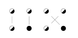
TikZ Diagramm

Hier ein kleiner Schnipsel TikZ, den ich für die Beantwortung einer LaTeX-Frage geschrieben habe.

\documentclass[fontsize=12pt]{scrartcl}
\usepackage{wasysym}
\usepackage{tikz}
\usepackage[right]{showlabels}
\usetikzlibrary{positioning}
\usepackage{graphicx} 
 
\newcommand{\half}{\rotatebox{-45}{\Huge\RIGHTcircle}}
\newcommand{\full}{\Huge\CIRCLE}
 
\begin{document}  
\begin{center}
\begin{tikzpicture}[x=20mm,y=20mm]
 
\node at (0,0) (a1)  {\half};
\node at (1,0)  (a2) {\half};
\node at (2,0) (a3) {\half};
\node at (3,0) (a4) {\half};
 
\node at (0,-1) (b1)  {\half};
\node at (1,-1) (b2){\full};
\node at (2,-1) (b3)  {\half};
\node at (3,-1) (b4) {\full};
 
\draw (a1) -- (b1);
\draw (a2) -- (b2);
\draw (a3) -- (b4);
\draw (a4) -- (b3);
 
 
\end{tikzpicture}
\end{center}
 
\end{document}