Archive for the ‘Statistik & Zahlen’ Category.
2021-01-17, 12:27
Im Beitrag „CSV-Dateien mit speziellen Spaltentrennern in Python laden“ hatte ich gezeigt, wie man mit BS4 Dateien aus Webseiten extrahieren und abspeichern kann, um sie dann in pandas weiterzuverarbeiten. Es geht auch ohne den Umweg der CSV-Datei, wenn man die StringIO Klasse aus dem io Modul nutzt.
Wir laden das Modul und instanziieren dann ein Objekt der Klasse mit dem von BS4 gefundenen Datensatz. Diese Objekt wird dann anstelle des Pfades der CSV-Datei an die pd.read_csv() Funktion übergeben.
import pandas as pd
import requests
from bs4 import BeautifulSoup
from io import StringIO
headers = {
'Access-Control-Allow-Origin': '*',
'Access-Control-Allow-Methods': 'GET',
'Access-Control-Allow-Headers': 'Content-Type',
'Access-Control-Max-Age': '3600',
'User-Agent': 'Mozilla/5.0 (X11; Ubuntu; Linux x86_64; rv:52.0) Gecko/20100101 Firefox/52.0'
}
url = "http://www.statistics4u.com/fundstat_eng/data_fluriedw.html"
req = requests.get(url, headers)
soup = BeautifulSoup(req.content, 'html.parser')
data=soup.find('pre').contents[0]
str_object = StringIO(data)
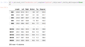
df = pd.read_csv(str_object,engine='python',skiprows=5,delim_whitespace=True)
print(df) |
import pandas as pd
import requests
from bs4 import BeautifulSoup
from io import StringIO
headers = {
'Access-Control-Allow-Origin': '*',
'Access-Control-Allow-Methods': 'GET',
'Access-Control-Allow-Headers': 'Content-Type',
'Access-Control-Max-Age': '3600',
'User-Agent': 'Mozilla/5.0 (X11; Ubuntu; Linux x86_64; rv:52.0) Gecko/20100101 Firefox/52.0'
}
url = "http://www.statistics4u.com/fundstat_eng/data_fluriedw.html"
req = requests.get(url, headers)
soup = BeautifulSoup(req.content, 'html.parser')
data=soup.find('pre').contents[0]
str_object = StringIO(data)
df = pd.read_csv(str_object,engine='python',skiprows=5,delim_whitespace=True)
print(df)
Uwe Ziegenhagen likes LaTeX and Python, sometimes even combined.
Do you like my content and would like to thank me for it? Consider making a small donation to my local fablab, the Dingfabrik Köln. Details on how to donate can be found here Spenden für die Dingfabrik.
More Posts - Website
2021-01-17, 11:58
Hier ein Beispiel, wie man Bilder für eine Animation mit matplotlib erstellen kann, adaptiert von im Netz gefundenen Code
Der folgende Python-Code erzeugt 720 einzelne Bilder und legt diese im Dateisystem ab. Mittels magick -quality 100 *.png outputfile.mpeg werden dann die Bilder zu einem MPEG-Video kombiniert. Hinweis: Nur unter Windows heißt der Befehl „magick“ da „convert“ auch ein Systemprogramm ist.
import matplotlib.pyplot as plt
import pandas as pd
import seaborn as sns
from mpl_toolkits.mplot3d import Axes3D

df = sns.load_dataset('iris')
sns.set(style = "darkgrid")

fig = plt.figure()
fig.set_size_inches(16, 9)

ax = fig.add_subplot(111, projection = '3d')

x = df['sepal_width']
y = df['sepal_length']
z = df['petal_width']

ax.set_xlabel("sepal_width")
ax.set_ylabel("sepal_lesngth")
ax.set_zlabel("petal_width")

c = {'setosa':'red', 'versicolor':'blue', 'virginica':'green'}

ax.scatter(x, y, z,c=df['species'].apply(lambda x: c[x]))

for angle in range(0, 720):
    ax.view_init((angle+1)/10, angle)
    plt.draw()
    plt.savefig('r:/'+str(angle).zfill(3)+'.png')
Eine kürzere Version der Animation habe ich unter https://www.youtube.com/watch?v=gdgvXpq4k1w abgelegt.
Hinweise zu anderen Konvertierungsprogrammen gibt es unter anderem hier: https://www.andrewnoske.com/wiki/Convert_an_image_sequence_to_a_movie
Uwe Ziegenhagen likes LaTeX and Python, sometimes even combined.
Do you like my content and would like to thank me for it? Consider making a small donation to my local fablab, the Dingfabrik Köln. Details on how to donate can be found here Spenden für die Dingfabrik.
More Posts - Website
2021-01-17, 00:21
Um einige Klassifikations-Algorithmen in Python ausprobieren zu können habe ich heute die Swiss Banknote Data von Flury und Riedwyl benötigt. Die Daten sind im Netz z.B. unter http://www.statistics4u.com/fundstat_eng/data_fluriedw.html verfügbar, ich wollte sie aber nicht manuell einladen müssen.
Mit dem folgenden Code, adaptiert von https://hackersandslackers.com/scraping-urls-with-beautifulsoup/, kann man die Daten lokal abspeichern und dann in einen pandas Dataframe einladen.
import pandas as pd
import requests
from bs4 import BeautifulSoup

headers = {
    'Access-Control-Allow-Origin': '*',
    'Access-Control-Allow-Methods': 'GET',
    'Access-Control-Allow-Headers': 'Content-Type',
    'Access-Control-Max-Age': '3600',
    'User-Agent': 'Mozilla/5.0 (X11; Ubuntu; Linux x86_64; rv:52.0) Gecko/20100101 Firefox/52.0'
}

url = "http://www.statistics4u.com/fundstat_eng/data_fluriedw.html"
req = requests.get(url, headers)
soup = BeautifulSoup(req.content, 'html.parser')

a=soup.find('pre').contents[0]

with open('banknote.csv','wt') as data:
    data.write(a)

df = pd.read_csv('banknote.csv',engine='python',skiprows=5,delim_whitespace=True)
print(df) |
import pandas as pd
import requests
from bs4 import BeautifulSoup
headers = {
'Access-Control-Allow-Origin': '*',
'Access-Control-Allow-Methods': 'GET',
'Access-Control-Allow-Headers': 'Content-Type',
'Access-Control-Max-Age': '3600',
'User-Agent': 'Mozilla/5.0 (X11; Ubuntu; Linux x86_64; rv:52.0) Gecko/20100101 Firefox/52.0'
}
url = "http://www.statistics4u.com/fundstat_eng/data_fluriedw.html"
req = requests.get(url, headers)
soup = BeautifulSoup(req.content, 'html.parser')
a=soup.find('pre').contents[0]
with open('banknote.csv','wt') as data:
data.write(a)
df = pd.read_csv('banknote.csv',engine='python',skiprows=5,delim_whitespace=True)
print(df)
Uwe Ziegenhagen likes LaTeX and Python, sometimes even combined.
Do you like my content and would like to thank me for it? Consider making a small donation to my local fablab, the Dingfabrik Köln. Details on how to donate can be found here Spenden für die Dingfabrik.
More Posts - Website
2021-01-16, 20:49
Ich habe heute auf einer meiner Linux-Maschinen Jupyter Notebook installiert. Um die — für die Arbeit im lokalen Netz lästigen — Sicherheitsabfragen zu umgehen, habe ich mir ausgehend von https://stackoverflow.com/questions/41159797/how-to-disable-password-request-for-a-jupyter-notebook-session ein kleines Startskript geschrieben:
#! /bin/bash
jupyter notebook --ip='*' --NotebookApp.token='' --NotebookApp.password='' |
#! /bin/bash
jupyter notebook --ip='*' --NotebookApp.token='' --NotebookApp.password=''
Uwe Ziegenhagen likes LaTeX and Python, sometimes even combined.
Do you like my content and would like to thank me for it? Consider making a small donation to my local fablab, the Dingfabrik Köln. Details on how to donate can be found here Spenden für die Dingfabrik.
More Posts - Website
2021-01-16, 20:45
Mit cudf gibt es ein Paket, das pandas Datenstrukturen auf nvidia-Grafikkarten verarbeiten kann. Einen i7 3770 mit 24 GB RAM habe ich jetzt mit einer CUDA-fähigen Grafikkarte (Typ Quadro P400) ausgestattet, damit ich damit rumspielen arbeiten kann. Unter https://towardsdatascience.com/heres-how-you-can-speedup-pandas-with-cudf-and-gpus-9ddc1716d5f2 findet man passende Beispiele, diese habe ich in einem Jupyter-Notebook laufenlassen.
Ein Geschwindigkeitszuwachs ist erkennbar, insbesondere bei der Matrix-Größe aus dem verlinkten Beispiel war die CUDA-Variante mehr als 3x so schnell wie die CPU-Variante. Das Merge mit der vollen Matrix-Größe lief bei mir leider nicht, da limitieren vermutlich die 2 GB RAM, die die P400 bietet.
Uwe Ziegenhagen likes LaTeX and Python, sometimes even combined.
Do you like my content and would like to thank me for it? Consider making a small donation to my local fablab, the Dingfabrik Köln. Details on how to donate can be found here Spenden für die Dingfabrik.
More Posts - Website
2021-01-10, 19:19
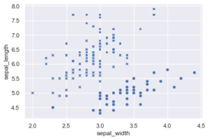
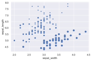
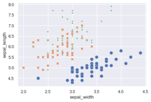
Im letzten Beitrag hatten wir mit hue die Zugehörigkeit der Iris Data Orchideen dargestellt, Seaborn besitzt aber mit style und size noch weitere Möglichkeiten der Unterscheidung. style nutzt dabei verschiedene Symbole, size unterschiedliche Punktgrößen. Die verschiedenen Optionen können auch kombiniert werden.
import seaborn as sns
sns.set(style = "darkgrid")
iris=sns.load_dataset('iris')

sns.scatterplot(
    x=iris['sepal_width'],
    y=iris['sepal_length'],
    style=iris['species'],
    legend=False
) |
import seaborn as sns
sns.set(style = "darkgrid")
iris=sns.load_dataset('iris')
sns.scatterplot(
x=iris['sepal_width'],
y=iris['sepal_length'],
style=iris['species'],
legend=False
)
import seaborn as sns
sns.set(style = "darkgrid")
iris=sns.load_dataset('iris')

sns.scatterplot(
    x=iris['sepal_width'],
    y=iris['sepal_length'],
    size=iris['species'],
    legend=False
) |
import seaborn as sns
sns.set(style = "darkgrid")
iris=sns.load_dataset('iris')
sns.scatterplot(
x=iris['sepal_width'],
y=iris['sepal_length'],
size=iris['species'],
legend=False
)
import seaborn as sns
sns.set(style = "darkgrid")
iris=sns.load_dataset('iris')

sns.scatterplot(
    x=iris['sepal_width'],
    y=iris['sepal_length'],
    hue=iris['species'],
    style=iris['species'],
    size=iris['species'],
    legend=False
) |
import seaborn as sns
sns.set(style = "darkgrid")
iris=sns.load_dataset('iris')
sns.scatterplot(
x=iris['sepal_width'],
y=iris['sepal_length'],
hue=iris['species'],
style=iris['species'],
size=iris['species'],
legend=False
)
Uwe Ziegenhagen likes LaTeX and Python, sometimes even combined.
Do you like my content and would like to thank me for it? Consider making a small donation to my local fablab, the Dingfabrik Köln. Details on how to donate can be found here Spenden für die Dingfabrik.
More Posts - Website
2021-01-09, 20:37
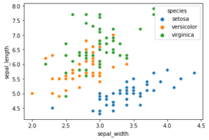
Hier ein einfaches Beispiel für einen Scatterplot mit Python und dem Seaborn Modul. Das Beispiel nutzt den bekannten Iris-Datensatz von R. Fisher, der gut für Klassifikationstechniken genutzt werden kann.
import seaborn as sns

iris=sns.load_dataset('iris')

sns.scatterplot(x=iris['sepal_width'],y=iris['sepal_length'],hue=iris['species']) |
import seaborn as sns
iris=sns.load_dataset('iris')
sns.scatterplot(x=iris['sepal_width'],y=iris['sepal_length'],hue=iris['species'])
Uwe Ziegenhagen likes LaTeX and Python, sometimes even combined.
Do you like my content and would like to thank me for it? Consider making a small donation to my local fablab, the Dingfabrik Köln. Details on how to donate can be found here Spenden für die Dingfabrik.
More Posts - Website
2020-06-07, 07:06
Per Zufall bin ich vor einigen Tagen auf ein Juwel im Steam-Shop gestoßen: „while True learn()“. Es ist kein Spiel im klassischen Sinne, sondern mehr eine Simulation zum Lernen von KL/ML-Algorithmen.
Die Geschichte ist schnell erzählt: Programmierer programmiert, kommt nicht weiter, seine Katze übernimmt und erklärt ihm in Katzensprache, was er tun muss. Da er kein Katzisch spricht, baut er mit Hilfe aus dem Netz schrttweise ein System zur Verständigung mit der Mieze.
Das Spiel geht anfangs recht einfach los, ein oder zwei Blöcke positionieren, Verbindungslinien setzen, los.
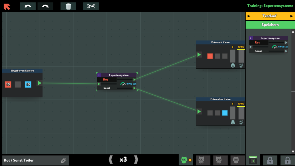
Über zeitliche Einschränkungen und Kostendruck kommt man aber schnell an den Punkt, an dem man denken muss.
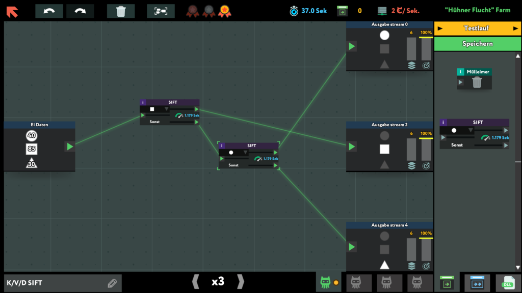
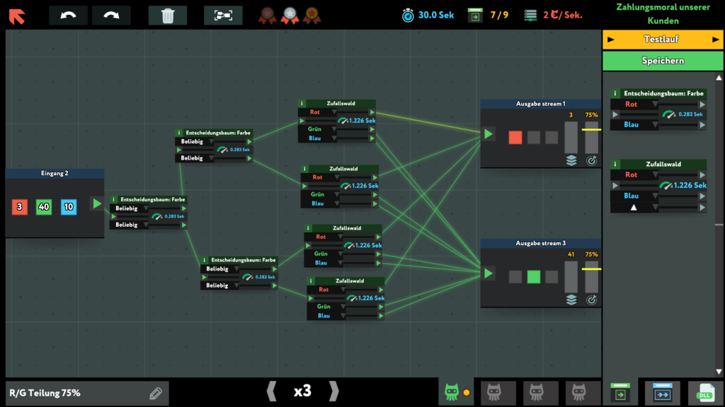
Von mir eine absolute Empfehlung!
Uwe Ziegenhagen likes LaTeX and Python, sometimes even combined.
Do you like my content and would like to thank me for it? Consider making a small donation to my local fablab, the Dingfabrik Köln. Details on how to donate can be found here Spenden für die Dingfabrik.
More Posts - Website
2017-03-25, 08:09
One of the many approximations of Pi is the Gregory-Leibniz series (image source Wikipedia):

Here is an implementation in Python:
# -*- coding: utf-8 -*-
"""
Created on Sat Mar 25 06:52:11 2017
@author: Uwe Ziegenhagen
"""

sum = 0
factor = -1

for i in range(1, 640000, 2):
        sum = sum + factor * 1/i
        factor *= -1
        # print(sum)

print(-4*sum) |
# -*- coding: utf-8 -*-
"""
Created on Sat Mar 25 06:52:11 2017
@author: Uwe Ziegenhagen
"""
sum = 0
factor = -1
for i in range(1, 640000, 2):
sum = sum + factor * 1/i
factor *= -1
# print(sum)
print(-4*sum)
Uwe Ziegenhagen likes LaTeX and Python, sometimes even combined.
Do you like my content and would like to thank me for it? Consider making a small donation to my local fablab, the Dingfabrik Köln. Details on how to donate can be found here Spenden für die Dingfabrik.
More Posts - Website
2017-03-14, 07:59
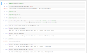
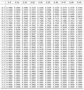
Here’s a simple example how one can generate a normal distribution table with Python and scipy so that it can be imported into LaTeX.
Example-03.zip
# -*- coding: utf-8 -*-
"""
Created on Mon Mar 13 21:14:17 2017
@author: Uwe Ziegenhagen, ziegenhagen@gmail.com

Creates a CDF table for the standard normal distribution

use booktabs package in the preamble and put
the generated numbers inside (use only one backslash!)

\\begin{tabular}{r|cccccccccc} \\toprule
<output here>
\\end{tabular}
"""

from scipy.stats import norm

print(norm.pdf(0))
print(norm.cdf(0),'\r\n')

horizontal = range(0,10,1)
vertikal = range(0,37)

header = ''
for i in horizontal:
    header = header + '& ' + str(i/100)

print(header, '\\\\ \\midrule')

for j in vertikal:
    x = j/10
    print('\\\\', x)
    for i in horizontal:
        y = x + i/100
        print('& ', "{:10.4f}".format(norm.cdf(y),4))


print('\\\\ \\bottomrule \r\n') |
# -*- coding: utf-8 -*-
"""
Created on Mon Mar 13 21:14:17 2017
@author: Uwe Ziegenhagen, ziegenhagen@gmail.com
Creates a CDF table for the standard normal distribution
use booktabs package in the preamble and put
the generated numbers inside (use only one backslash!)
\\begin{tabular}{r|cccccccccc} \\toprule
<output here>
\\end{tabular}
"""
from scipy.stats import norm
print(norm.pdf(0))
print(norm.cdf(0),'\r\n')
horizontal = range(0,10,1)
vertikal = range(0,37)
header = ''
for i in horizontal:
header = header + '& ' + str(i/100)
print(header, '\\\\ \\midrule')
for j in vertikal:
x = j/10
print('\\\\', x)
for i in horizontal:
y = x + i/100
print('& ', "{:10.4f}".format(norm.cdf(y),4))
print('\\\\ \\bottomrule \r\n')
Uwe Ziegenhagen likes LaTeX and Python, sometimes even combined.
Do you like my content and would like to thank me for it? Consider making a small donation to my local fablab, the Dingfabrik Köln. Details on how to donate can be found here Spenden für die Dingfabrik.
More Posts - Website